Development

In this section Everest development decisions are documented.

Architecture

The everest application is split into two components, a server component and a client component.

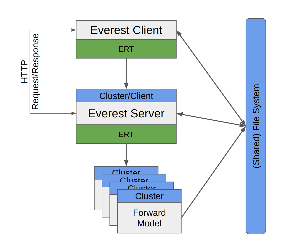
Fig. 2 Everest architecture

Every time an optimization instance is ran by a user, the client component of the application spawns an instance of the server component, which is started either on a cluster node using LSF (when the queue_system is defined to be lsf) or on the client’s machine (when the queue_system is defined to be local).

Communication between the two components is done via an HTTP API.

Server HTTP API

The Everest server component supports the following HTTP requests API. The Everest server component was designed as an internal component that will be available as long as the optimization process is running.

Table 1 Server HTTP API

Method	Endpoint	Description
GET	‘/’	Check server is online
GET	‘/sim_progress’	Simulation progress information
GET	‘/opt_progress’	Optimization progress information
POST	‘/stop’	Signal everest optimization run termination. It will be called by the client when the optimization needs to be terminated in the middle of the run

EVEREST vs. ERT data models

EVEREST uses ERT for running an experiment. An experiment contains several batches (i.e., ensembles). An ensemble / batch contains inputs & computed outputs for several realizations, denoted as simulations in EVEREST. EVEREST controls are mapped to ERT parameters and serve as input to each forward model evaluation. ERT generates responses for each forward model evaluation in the batch. ERT writes these responses to storage in the simulation_results folder (per batch and per realization). These responses are mapped to objectives and constraints in EVEREST and forwarded to ropt (i.e., the optimizer). To summarize, every forward model evaluation for a single set of inputs/parameters (controls) and generated outputs/responses (objectives / constraints) constitutes an ERT realization (simulation in EVEREST).

For controls in EVEREST, there is a distinction between unperturbed controls (i.e., controls of the current best solution yielding the best objective function value(s), see also The optimization process) and perturbed controls (i.e., required to calculate the gradient). Furthermore, when performing robust optimization a batch contains multiple model_realizations (denoted by <MODEL_ID>). A model_realization is a set of static variables (i.e., not changing during the optimization) which affect the response of the underlying optimized model (NOTE: model_realization is not the same as an ERT realization; see also Robust Optimization: Stochastic Simplex Gradients (StoSAG)). Each model_realization can contain several simulations (i.e., forward model runs). This is the key difference between the hierarchical data model of EVEREST and ERT (Fig 3). NOTE: <MODEL_ID> (or <GEO_ID> due to legacy reasons) is inserted (and substituted) in the run_path for each model_realization.

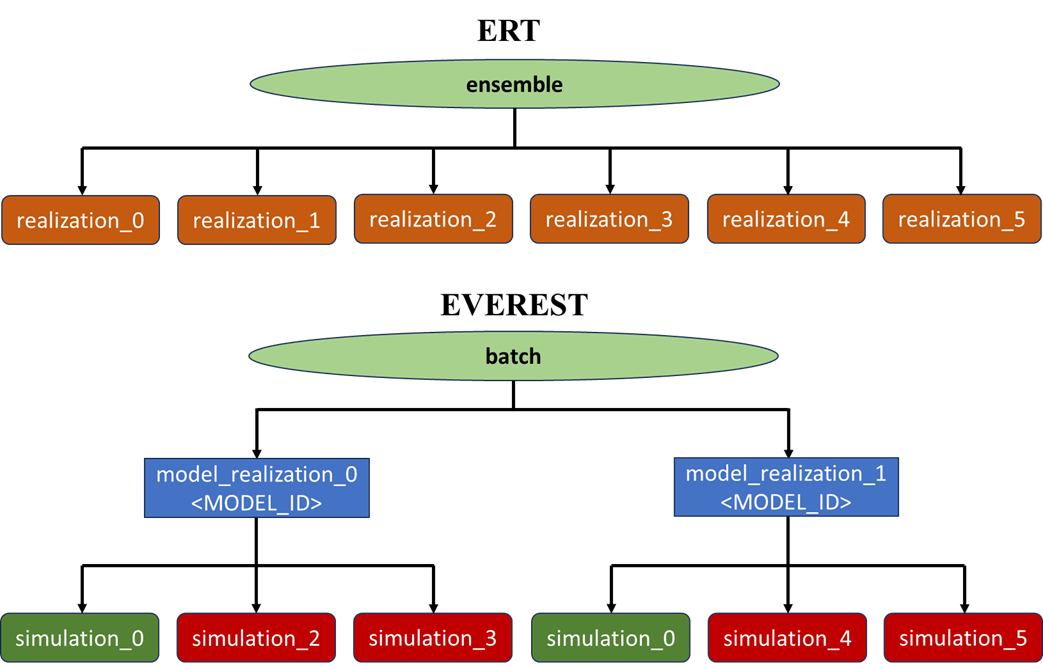
Fig. 3 Difference between ensemble in ERT and batch in EVEREST.

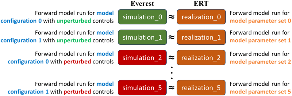
Fig. 4 Different meaning of realization and simulation.

The mapping from data models in EVEREST to ERT is done in EVEREST, meaning realization (ERT) to <MODEL_ID> and pertubation-number (EVEREST). Batches in EVEREST can contain several different configurations depending on the algorithm used. Gradient-based algorithms can have a single function evaluation (unperturbed controls) per <MODEL_ID>, a set of perturbed controls per <MODEL_ID> to evaluate the gradient, or both. Derivative-free methods can have several function evaluations per <MODEL_ID> and no perturbed controls. NOTE: the optimizer may decide that some <MODEL_ID> are not needed, these are then skipped and the output from ropt will reflect this (i.e., less <MODEL_ID>`s in the `batch results than expected).

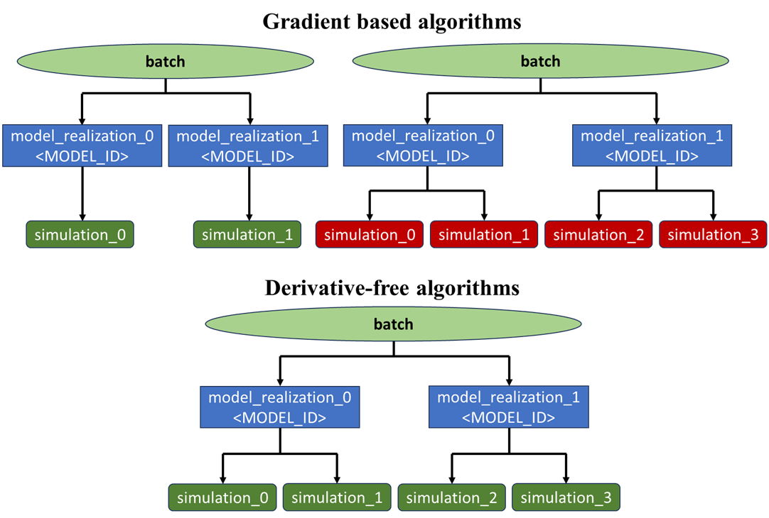
Fig. 5 Three other possible configurations of EVEREST batches in the context of gradient-based and gradient-free optimization algorithms.